44 excel chart change all data labels at once

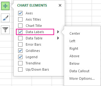
How to Add Total Data Labels to the Excel Stacked Bar Chart Step 4: Right click your new line chart and select "Add Data Labels" Step 5: Right click your new data labels and format them so that their label position is "Above"; also make the labels bold and increase the font size. Step 6: Right click the line, select "Format Data Series"; in the Line Color menu, select "No line" Step 7 ... How to add or move data labels in Excel chart? - ExtendOffice In Excel 2013 or 2016. 1. Click the chart to show the Chart Elements button . 2. Then click the Chart Elements, and check Data Labels, then you can click the arrow to choose an option about the data labels in the sub menu. See screenshot: In Excel 2010 or 2007. 1. click on the chart to show the Layout tab in the Chart Tools group. See ...

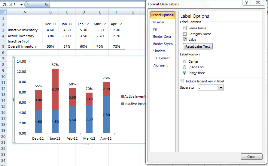
Format Data Labels in Excel- Instructions - TeachUcomp, Inc. To format data labels in Excel, choose the set of data labels to format. To do this, click the "Format" tab within the "Chart Tools" contextual tab in the Ribbon. Then select the data labels to format from the "Chart Elements" drop-down in the "Current Selection" button group. Then click the "Format Selection" button that ...

Excel chart change all data labels at once

Insert a chart from an Excel spreadsheet into Word Keep Source Formatting & Link Data. Keeps the Excel theme. Keeps the chart linked to the original workbook. To update the chart automatically, change the data in the original workbook. You also can select Chart Tools> Design > Refresh Data. Picture. Becomes a picture. You can’t update the data or edit the chart, but you can adjust the chart ... Adding rich data labels to charts in Excel 2013 | Microsoft 365 Blog Putting a data label into a shape can add another type of visual emphasis. To add a data label in a shape, select the data point of interest, then right-click it to pull up the context menu. Click Add Data Label, then click Add Data Callout . The result is that your data label will appear in a graphical callout. How to format multiple charts quickly - Excel Off The Grid Here is the chart format we wish to copy: We can click anywhere on the chart. Then click Home -> Copy (or Ctrl + C) Now click on the chart you want to format. Then click Home -> Paste Special. From the Paste Special window select "Formats", then click OK. Ta-dah! With just a few click you can quickly change the format of a chart.

Excel chart change all data labels at once. Edit titles or data labels in a chart - support.microsoft.com You can also place data labels in a standard position relative to their data markers. Depending on the chart type, you can choose from a variety of positioning options. On a chart, do one of the following: To reposition all data labels for an entire data series, click a data label once to select the data series. Excel changes multiple series colors at once sub formatseriesthesame() if activechart is nothing then msgbox "select a chart and try again!", vbexclamation goto exitsub end if with activechart dim icolor as long icolor = .seriescollection(2).format.line.forecolor.rgb dim iseries as long for iseries = 3 to .seriescollection.count .seriescollection(iseries).format.line.forecolor.rgb = icolor … change all data labels - Excel Help Forum For a new thread (1st post), scroll to Manage Attachments, otherwise scroll down to GO ADVANCED, click, and then scroll down to MANAGE ATTACHMENTS and click again. Now follow the instructions at the top of that screen. New Notice for experts and gurus: Change the labels in an Excel data series | TechRepublic Select B15:D15. Click the Chart Wizard button in the Standard toolbar. Click Next. Click the Series tab. Click the Window Shade button in the Category (X) Axis. Labels box. Select B3:D3 to select ...

Custom Data Labels with Colors and Symbols in Excel Charts - [How To ... Step 4: Select the data in column C and hit Ctrl+1 to invoke format cell dialogue box. From left click custom and have your cursor in the type field and follow these steps: Press and Hold ALT key on the keyboard and on the Numpad hit 3 and 0 keys. Let go the ALT key and you will see that upward arrow is inserted. Add a DATA LABEL to ONE POINT on a chart in Excel Method — add one data label to a chart line Steps shown in the video above: Click on the chart line to add the data point to. All the data points will be highlighted. Click again on the single point that you want to add a data label to. Right-click and select ' Add data label ' This is the key step! Select all Data Labels at once - Microsoft Community The Tab key will move among chart elements. Click on a chart column or bar. Click again so only 1 is selected. Press the Tab key. Each column or bar in the series is selected in turn, then it moves to selecting each data label in the series. Author of "OOXML Hacking - Unlocking Microsoft Office's Secrets", ebook now out Excel charts: add title, customize chart axis, legend and data labels Click anywhere within your Excel chart, then click the Chart Elements button and check the Axis Titles box. If you want to display the title only for one axis, either horizontal or vertical, click the arrow next to Axis Titles and clear one of the boxes: Click the axis title box on the chart, and type the text.

Move and Align Chart Titles, Labels, Legends with the Arrow Keys Select the element in the chart you want to move (title, data labels, legend, plot area). On the add-in window press the "Move Selected Object with Arrow Keys" button. This is a toggle button and you want to press it down to turn on the arrow keys. Press any of the arrow keys on the keyboard to move the chart element. Multiple Time Series in an Excel Chart - Peltier Tech 12/08/2016 · I recently showed several ways to display Multiple Series in One Excel Chart.The current article describes a special case of this, in which the X values are dates. Displaying multiple time series in an Excel chart is not difficult if all the series use the same dates, but it becomes a problem if the dates are different, for example, if the series show monthly and … How to Create a Timeline Chart in Excel - Automate Excel In order to polish up the timeline chart, you can now add another set of data labels to track the progress made on each task at hand. Right-click on any of the columns representing Series “Hours Spent” and select “Add Data Labels.” Once there, right-click on any of the data labels and open the Format Data Labels task pane. Then, insert ... Create a multi-level category chart in Excel - ExtendOffice 16. Right click the chart and select Change Series Chart Type in the right-clicking menu. 17. In the Change Chart Type dialog box, specify the Chart Type as “Scatter” for the new series you added in step 15, and then click OK. Now the chart is displayed as the below screenshot shown. 18. Right click the chart and click Select Data in the ...

How to Add Data Labels to your Excel Chart in Excel 2013 - YouTube

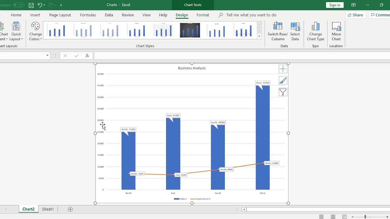
Excel Chart - Selecting and updating ALL data labels Selection.ShowSeriesName = True Selection.ShowValue = False Next End With End Sub Worf Well-known Member Joined Oct 30, 2011 Messages 4,205 Jan 9, 2013 #4 The following procedure accomplished your requirement; tell me how it works out for you: - Right-click a "point" in the series, which actually will be a bar piece - Choose add data labels

excel - How do I update the data label of a chart? - Stack Overflow

Excel Gauge Chart Template - Free Download - How to Create Move the labels to the appropriate places above the gauge chart. Change the chart title. Bonus Step for the Tenacious: Add a text box with your actual data value. Here is a quick and dirty tip on making the speedometer chart more informative as well as pleasing to the eye. Let’s add a text box that will display the actual value of the pointer.

Format Number Options for Chart Data Labels in Excel 2011 for Mac

change format for all data series in chart [SOLVED] Re: change format for all data series in chart. It might depend on the kind of format change you are trying to do. The only "chart wide" command I can think of is the "change chart type" command. So, if you have a scatter chart with markers and no lines and you want to add lines to each data series, you could go into the change chart type, and ...

Excel Charts | How to Create a Chart in Excel | MS Excel in Hindi

How to add data labels from different column in an Excel chart? Click any data label to select all data labels, and then click the specified data label to select it only in the chart. 3. Go to the formula bar, type =, select the corresponding cell in the different column, and press the Enter key. See screenshot: 4. Repeat the above 2 - 3 steps to add data labels from the different column for other data points.

How to Add Data Labels in Excel - Excelchat | Excelchat

How to set multiple series labels at once - Microsoft Tech Community Click anywhere in the chart. On the Chart Design tab of the ribbon, in the Data group, click Select Data. Click in the 'Chart data range' box. Select the range containing both the series names and the series values. Click OK. If this doesn't work, press Ctrl+Z to undo the change. 0 Likes Reply Nathan1123130 replied to Hans Vogelaar

Custom Data Labels with Colors and Symbols in Excel Charts - [How To] - PakAccountants.com

Excel chart changing all data labels from value to series name ... By selecting chart then from layout->data labels->more data labels options ->label options ->label contains-> (select)series name, I can only get one series name replacing its respective label values. For more than hundred series stacked in columns i want them all to be changed at once, is there any way out? why it does not change them all at once?

Move data labels - Office Support

Dynamically Label Excel Chart Series Lines - My Online Training … 26/09/2017 · To modify the axis so the Year and Month labels are nested; right-click the chart > Select Data > Edit the Horizontal (category) Axis Labels > change the ‘Axis label range’ to include column A. Step 2: Clever Formula. The Label Series Data contains a formula that only returns the value for the last row of data.

time series - PHPExcel X-Axis labels missing on scatter plot - Stack Overflow

Make Excel charts easier to read by adjusting data markers Select the chart, then click. on the data series. Go to Format | Selected Data Series. On the Options tab, select the Vary Colors By Point check box. Click OK. Now each point has its own ...

Formula Friday - Using Formulas To Add Custom Data Labels To Your Excel Chart - How To Excel At ...

Change the position of data labels automatically Click the chart outside of the data labels that you want to change. Click one of the data labels in the series that you want to change. On the Format menu, click Selected Data Labels, and then click the Alignment tab. In the Label position box, click the location you want. previous page start next page.

How to remove blank rows in Excel to tidy up your sheet - Business Insider

How to change chart axis labels' font color and size in Excel? We can easily change all labels' font color and font size in X axis or Y axis in a chart. Just click to select the axis you will change all labels' font color and size in the chart, and then type a font size into the Font Size box, click the Font color button and specify a font color from the drop down list in the Font group on the Home tab. See below screen shot:

Creating a chart with dynamic labels - Microsoft Excel 2016

Comparison Chart in Excel | Adding Multiple Series Under Same … This window helps you modify the chart as it allows you to add the series (Y-Values) as well as Category labels (X-Axis) to configure the chart as per your need. Under Legend Entries ( S eries) inside the Select Data Source window, you need to select the …

Do My Excel Blog: How to design a multiple clustered bar chart series in Excel

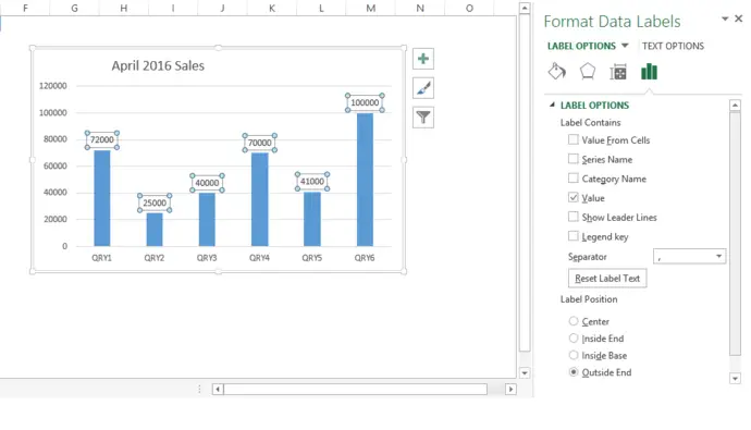
Change the format of data labels in a chart To get there, after adding your data labels, select the data label to format, and then click Chart Elements > Data Labels > More Options. To go to the appropriate area, click one of the four icons ( Fill & Line, Effects, Size & Properties ( Layout & Properties in Outlook or Word), or Label Options) shown here.

How To Add Data Labels To A Chart in Microsoft Excel - YouTube

Modify Excel Chart Data Range | CustomGuide You can also change the order of data in the chart without changing the order of the source data. Select the chart. Click the Design tab. Click the Select Data button. From the Select Data Source dialog box, select the data series you want to move. Click the Move Up or Move down button. Click OK . The chart is updated to display the new order ...

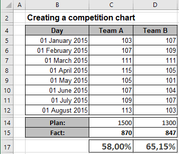
How to Change Excel Chart Data Labels to Custom Values?

how to add data labels into Excel graphs — storytelling with data To adjust the number formatting, navigate back to the Format Data Label menu and scroll to the Number section at the bottom. I'll choose Number in the Category drop-down and change Decimal places to 0 (side note: checking the Linked to source box is a good option if you want the labels to reformat when the formatting of the underlying source data changes).

How to Create a Chart in Microsoft Excel - Tech Support

How to Change Excel Chart Data Labels to Custom Values? - Chandoo.org Now, click on any data label. This will select "all" data labels. Now click once again. At this point excel will select only one data label. Go to Formula bar, press = and point to the cell where the data label for that chart data point is defined. Repeat the process for all other data labels, one after another. See the screencast. Points to note:

How-to Put Percentage Labels on Top of a Stacked Column Chart - Excel Dashboard Templates

How to Customize Your Excel Pivot Chart Data Labels - dummies Excel displays the Format Data Labels pane. Check the box that corresponds to the bit of pivot table or Excel table information that you want to use as the label. For example, if you want to label data markers with a pivot table chart using data series names, select the Series Name check box. If you want to label data markers with a category ...

Get more control over chart data labels in Google Sheets | The Noc Group

Add data labels and callouts to charts in Excel 365 - EasyTweaks.com Step #3: Format the data labels. Excel also gives you the option of formatting the data labels to suit your desired look if you don't like the default. To make changes to the data labels, right-click within the chart and select the "Format Labels" option.

Share :